| unvotes | |||
|---|---|---|---|
| rcid | country | country_code | vote |
| 381 | Paraguay | PY | yes |
| 5645 | Tanzania | TZ | yes |
| 4856 | Barbados | BB | yes |
| 3653 | South Korea | KR | yes |
| 4983 | China | CN | yes |
| 3316 | Philippines | PH | yes |
| 2948 | Egypt | EG | yes |
| 3054 | Luxembourg | LU | abstain |
| 2601 | Chile | CL | yes |
| 4742 | Tunisia | TN | yes |
PA 8: United Nations Voting Records
This task is complex. It requires many different types of abilities. Everyone will be good at some of these abilities but nobody will be good at all of them. In order to solve this puzzle, you will need to use the skills of each member of your group.
Groupwork Protocols
During the Practice Activity, you and your partner will alternate between two roles—Computer and Coder.
When you are the Computer, you will type into the Quarto document in RStudio. However, you do not type your own ideas. Instead, you type what the Coder tells you to type. You are permitted to ask the Coder clarifying questions, and, if both of you have a question, you are permitted to ask the professor. You are expected to run the code provided by the Coder and, if necessary, to work with the Coder to debug the code. Once the code runs, you are expected to collaborate with the Coder to write code comments that describe the actions taken by your code.
When you are the Coder, you are responsible for reading the instructions / prompts and directing the Computer what to type in the Quarto document. You are responsible for managing the resources your group has available to you (e.g., cheatsheet, textbook). If necessary, you should work with the Computer to debug the code you specified. Once the code runs, you are expected to collaborate with the Computer to write code comments that describe the actions taken by your code.
Here are more details of the Pair Programming Protocols
Note
The partner was born the furthest away from CSUMB will start as the Computer (typing and listening to instructions from the Coder).
Group Norms
Remember, your group is expected to adhere to the following norms:
- Be curious. Don’t correct.
- Be open minded.
- Ask questions rather than contribute.
- Respect each other.
- Allow each teammate to contribute to the activity through their role.
- Do not divide the work.
- No cross talk with other groups.
- Communicate with each other!
Goals for the Activity
- Join multiple data tables together by a common variable(s)
- Create new data sets through the joining of data from various sources
- Combine
joinfunctions with othertidyversefunctions
THROUGHOUT THE Activity be sure to follow the Style Guide by doing the following:
- load the appropriate packages at the beginning of the Quarto document
- use proper spacing
- add labels to all code chunks
- comment at least once in each code chunk to describe why you made your coding decisions
- add appropriate labels to all graphic axes
Setting up your Project
Your project should have the following components:
- completed pa-8-united-nations-voting-activity.qmd
- rendered file as
.html
Important
The original Computer should submit the zip file for the canvas quiz. The original Coder can just submit the rendered html file.
Computer - Be sure to share the final .qmd and .html file with the original Coder.
Data Description
The data this week comes from Harvard’s Dataverse by way of Mine Çetinkaya-Rundel, David Robinson, and Nicholas Goguen-Compagnoni.
Original Data citation: Erik Voeten “Data and Analyses of Voting in the UN General Assembly” Routledge Handbook of International Organization, edited by Bob Reinalda (published May 27, 2013). Available at SSRN: http://ssrn.com/abstract=2111149
It was featured on TidyTuesday
Here is each data set and its description (you might want to look at the Tidy Tuesday link for the tables already rendered)
unvotes.csv
| variable | class | description |
|---|---|---|
| rcid | double | The roll call id |
| country | character | Country name, by official English short name |
| country_code | character | 2-character ISO country code |
| vote | integer | Vote result as a factor of yes/abstain/no |
roll_calls.csv
| variable | class | description |
|---|---|---|
| rcid | integer | The roll call id |
| session | double | Session number. The UN holds one session per year; these started in 1946 |
| importantvote | integer | Whether the vote was classified as important by the U.S. State Department report “Voting Practices in the United Nations”. These classifications began with session 39 |
| date | double | Date of the vote, as a Date vector |
| unres | character | Resolution code |
| amend | integer | Whether the vote was on an amendment; coded only until 1985 |
| para | integer | Whether the vote was only on a paragraph and not a resolution; coded only until 1985 |
| short | character | Short description |
| descr | character | Longer description |
| roll_calls | ||||||||
|---|---|---|---|---|---|---|---|---|
| rcid | session | importantvote | date | unres | amend | para | short | descr |
| 6147 | 73 | NA | 2018-12-20 | R/73/240 | NA | NA | Towards a new international economic order : resolution / adopted by the General Assembly | A/73/251 22a - Globalization and interdependence. - GLOBALIZATION--INTERDEPENDENCE |
| 2588 | 38 | 0 | 1983-12-02 | R/38/83F | 0 | 0 | UNRWA | TO ASK ALL STATES TO MAKE CONTRIBUTIONS TO MEET THE INTERRUPTED NEEDS OF THE UN RELIEF AND WORKS AGENCY FOR PALESTINE REFUGEES AND TO URGE THE COMMISSIONER-GENERAL OF THE AGENCY TO RESUME THE INTERRUPTED GENERAL RATION DISTRIBUTION TO PALESTINE |
| 4579 | 59 | 0 | 2004-12-03 | R/59/65 | NA | NA | Prevention of arms race in outer space : resolution / adopte | Prevention of arms race in outer space : resolution / adopted by the General Assembly |
| 3670 | 47 | 1 | 1992-11-03 | R/47/19 | NA | NA | CUBA, U.S. EMBARGO | Necessity of ending the economic, commercial and financial embargo imposed by the United States against Cuba |
| 2025 | 34 | 0 | 1979-11-03 | R/34/52F | 0 | 0 | GAZA STRIP, REFUGEES | TO APPROVE A RESOLUTION CALLING UPON ISRAEL TO DESIST FROM REMOVAL AND RESETTLEMENT OF PALESTINIAN REFUGEES IN THE GAZA STRIP AND FROM DESTRUCTION OF THEIR SHELTERS. |
| 6025 | 52 | NA | 1997-12-09 | R/52/41 | NA | 1 | NA | The President: We have thus concluded this stage ofour consideration of agenda item 73. Agenda item 74 The risk of nuclear proliferation in the Middle East Report of the First Committee (A/52/603) 67th plenary meeting 9 December 1997 The President: The Assembly will now take a decision on the draft resolution recommended by the First Committee in paragraph 10 of its report in document A/52/603. A separate vote has been requested on the sixth preambular paragraph of the draft resolution. If there is no objection, I shall therefore put to the vote first the sixth preambular paragraph. A recorded vote has been requested. A |
| 3154 | 42 | 0 | 1987-11-02 | R/42/42H | NA | NA | DISARMAMENT WEEK | Disarmament Week |
| 3959 | 50 | 1 | 1995-12-06 | R/50/197 | NA | NA | HUMAN RIGHTS, SUDAN | Situation of human rights in the Sudan |
| 1647 | 30 | 0 | 1975-12-05 | R/30/3538 | 0 | 0 | CAPITAL FUND | TO CALL UPON ALL MEMBER STATES TO MAKE THEIR BEST EFFORTS TO OVERCOME CONSTRAINTS TO THE PROMPT PAYMENT EARLY IN EACH YEAR OF FULL ASSESSED CONTRIBUTIONS AND OF ADVANCES TO THE WORKING CAPITAL FUND. |
| 5844 | 63 | NA | 2008-12-24 | R/63/240 | NA | 1 | NA | The President (spoke in Spanish): I shall now put to the vote operative paragraph 5 of draft resolution XXV. A recorded vote has been requested. A |
issues.csv
| variable | class | description |
|---|---|---|
| rcid | integer | The roll call id |
| short_name | character | Two-letter issue codes |
| issue | integer | Descriptive issue name |
| issues | ||
|---|---|---|
| rcid | short_name | issue |
| 2091 | ec | Economic development |
| 5100 | hr | Human rights |
| 1104 | di | Arms control and disarmament |
| 9145 | ec | Economic development |
| 3355 | hr | Human rights |
| 4320 | di | Arms control and disarmament |
| 3333 | nu | Nuclear weapons and nuclear material |
| 5871 | nu | Nuclear weapons and nuclear material |
| 2832 | di | Arms control and disarmament |
| 4527 | hr | Human rights |
What variable(s) do each of these data frames have in common?
Data Exploration
Our goal today is to explore how various members (countries) in the United Nations vote. We have three data sets, what can we determine from each data set separately?
UN Votes
The first data set, unvotes contains data on the rcid which is the roll call id for the vote, the country/country code, and how the country voted. What can we learn from the data?
Comment on the following code, what is happening in each line? One way to approach seeing what each line does is to highlight the code from before the pipe of that line up to the data unvotes and use CTRL + ENTER to run just the highlighted lines.
unvotes |>
  count(country, vote) |> #comment
  group_by(country) |> #comment
  mutate(total = sum(n)) |> #comment
  mutate(prop_vote = n/total) |> #comment
  filter(country %in% c("United States", "Canada",
                        "Germany", "France",
                        "Italy", "Japan",
                        "United Kingdom")) |> #comment
  ggplot(aes(y = country, x = prop_vote,
             fill = vote)) + #comment
  geom_col(position = position_stack()) + #comment
  labs(y = "Group of Seven Countries",
       x = "Proportion of Votes",
       title = "Voting Record of the G7",
       fill = "Vote") + #comment
  theme_minimal() +  #comment
scale_fill_viridis_d(end = 0.8) 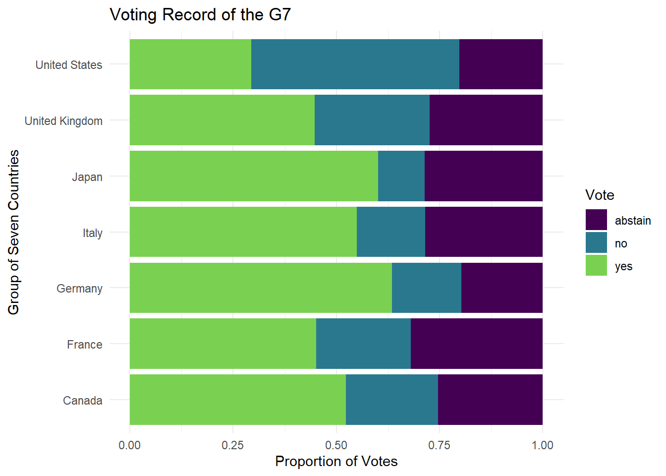
Describe what the graph above demonstrates above UN voting records for the G7.
Roll Calls
The second data set, roll_calls has more information on the type of vote, the importance, whether it was a resolution, and date of the vote.
roll_calls |>
  distinct(short)
# A tibble: 2,019 × 1
short
<chr>
1 AMENDMENTS, RULES OF PROCEDURE
2 SECURITY COUNCIL ELECTIONS
3 VOTING PROCEDURE
4 DECLARATION OF HUMAN RIGHTS
5 GENERAL ASSEMBLY ELECTIONS
6 ECOSOC POWERS
7 POST-WAR RECONSTRUCTION
8 U.N. MEMBERS, RELATIONS WITH SPAIN
9 TRUSTEESHIP AMENDMENTS
10 COUNCIL MEMBER TERM LENGTH
# ℹ 2,009 more rowsWhat does the code above do? What information does it provide? Is it useful? > Description of code results
We can use the individual data for roll_calls to look at the number of votes per year over time.
roll_calls |>
  mutate(year = lubridate::year(date)) |> #extracts the year from the date value and creates a new `year` column
  count(year) |> #counts how many votes there were per year assuming each line is an single voting instance
  ggplot(aes(x = year, y = n)) +
  geom_line() +
  labs(x = "Year", y = "Number of Votes",
       title = "UN Votes per Year") +
  theme_minimal()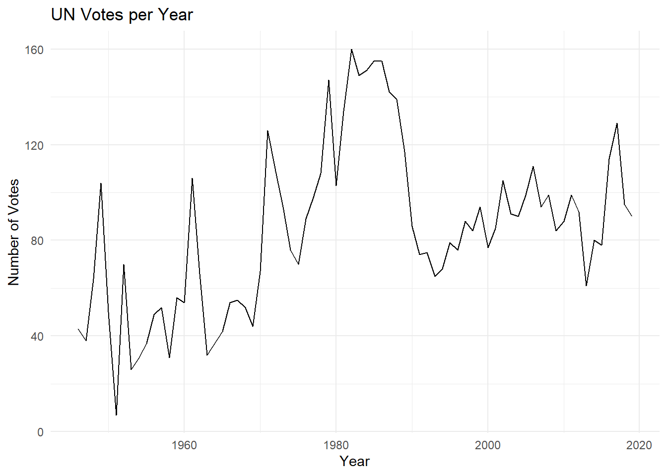
What information is missing from the above graphic that might be useful in understanding the issues the UN commonly votes on?
Issues
Finally we have the issues data which provides a more general description for each vote on specific issues. Note that not all issues are included in the data set, just the ones related to the 6 issues below:
issues |>
  count(issue) |>
  adorn_totals("row") #from janitor package
issue n
Arms control and disarmament 1092
Colonialism 957
Economic development 765
Human rights 1015
Nuclear weapons and nuclear material 855
Palestinian conflict 1061
Total 5745Notice the size of the issues data - it has 5745 rows, but if look at the distinct number of roll call identification numbers, you will see that there are 4099, meaning that more than one issue can be associated with the same roll call id/vote.
issues |>
  distinct(rcid) |>
  n_distinct()
[1] 4099Recall that in roll_call there are 6202 distinct roll call ids/votes, so the issues associated with issues do not represent all votes (i.e., there were other U.N. votes on other issues than our 6 chosen issues).
roll_calls |>
  distinct(rcid) |>
  n_distinct()
[1] 6202It would be helpful to use the issues data with the roll_calls data to be able to better understand the voting trends within the UN on these 6 issues. To do this, we need to join the data.
Votes Over Time
Now let’s join our data together to get a better idea of how the UN has voted over time.
First, look at the number of rows in issues and roll_calls - do they match? What does this indicate?
dim(issues)[1] 5745 3dim(roll_calls)[1] 6202 9Now let’s try joining the roll_calls with the issues data. Compare the following codes to join the data. Describe what each one does and how it differs from the others as a comment in the code chunk. You might need to reference the slides or reading for this week.
roll_calls |>
  left_join(issues, by = "rcid") #description of join
roll_calls |>
right_join(issues, by = "rcid") #description of joinroll_calls |>
full_join(issues, by = "rcid") #description of joinroll_calls |>
inner_join(issues, by = "rcid") #description of joinIf we are only interested in retaining the records associated with the issues labeled in that data frame, ignoring the other votes, which join should we use?
Now that we know how to join the data, we will use the following code to examine the the voting trends for three of the issues related to conflict/weapons.
Be sure to run the code via the green arrow on the code chunk, as the case_when() code can get finicky sometimes and claim an error about a comma in the code when it doesn’t exist. Comment on the code where indicated and add your chosen join function
roll_calls |>
 __________join(issues, by = "rcid") |>  #join roll_calls and issues so that just the votes related to the issues data are retained.
  mutate(issue_short = case_when(
    issue == "Arms control and disarmament" ~ "Arms Control",
    issue == "Nuclear weapons and nuclear material" ~ "Nuclear Weapons",
    issue == "Palestinian conflict" ~ "Palestinian Conflict",
    TRUE ~ issue)) |>   #what is happening in this mutate function?
  filter(issue_short %in% c("Arms Control",
                            "Nuclear Weapons",
                            "Palestinian Conflict")) |> #what are we doing here?
  mutate(year = lubridate::year(date)) |> #create a column `year` that contains the year value
  count(year,
        issue_short) |> #what does this line do?
  ggplot(aes(x = year,
             y = n,
             group = issue_short)) + #what does this line do?
  geom_line(aes(color = issue_short)) + #what does this line do?
  labs(x = "Year",
       y = "Number of Votes",
       title = "United Nations Votes per Year",
       subtitle = "Conflict and Arms Related Votes",
       color = "Voting Issue") +
  theme_minimal() +
  scale_color_viridis_d(end = 0.9)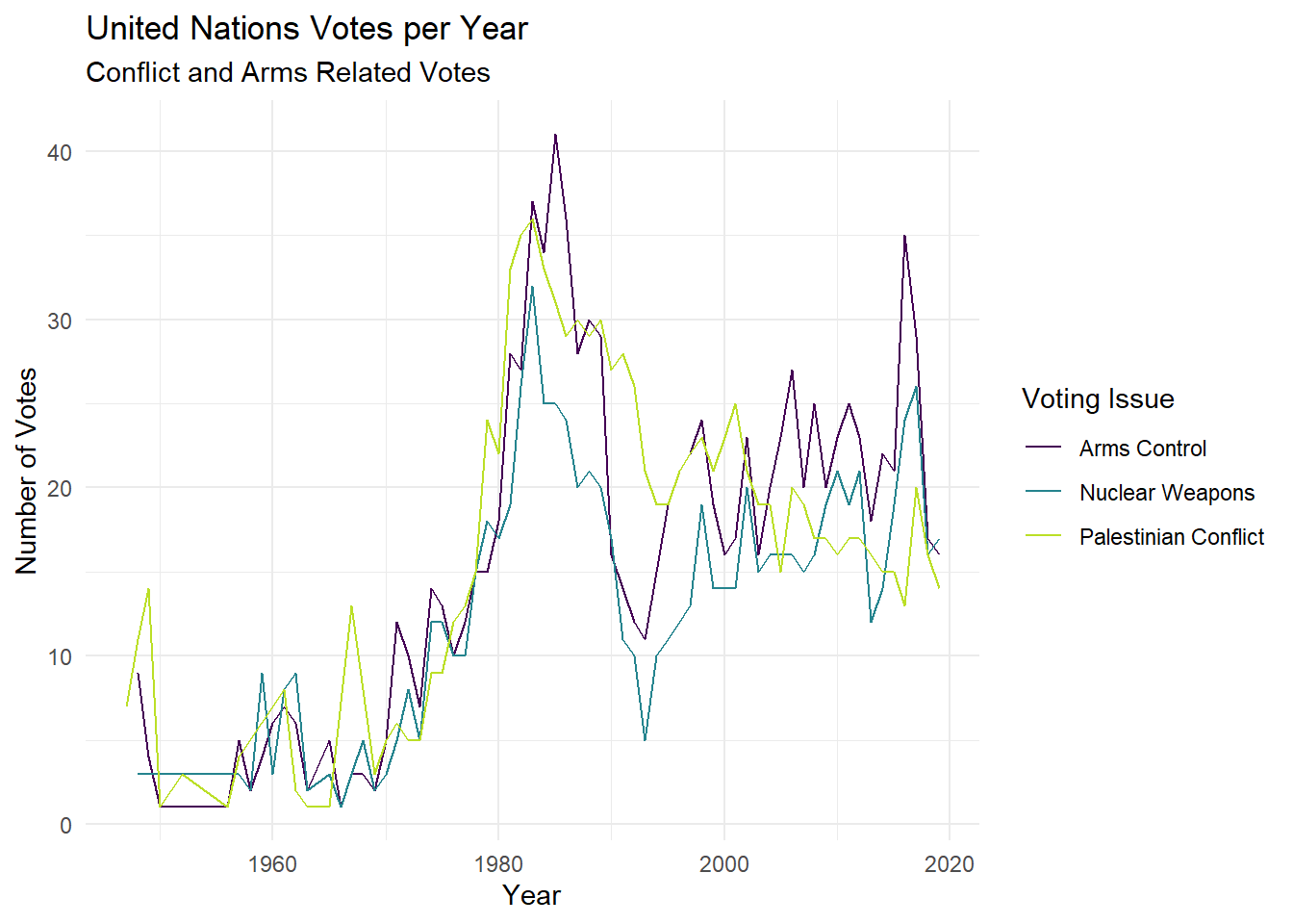
What do you notice? What do you wonder based on the graph created?
Joining all Data
We want to try create a visualization that compares the voting records of the US and Canada on the 6 major issues of interest. To do this, though, we need information from all three data set, unvotes, issues, and roll_calls
We want to join all three data sets together, maintaining only the votes for which we have identified the general issue (e.g., Nuclear War, Arms, Economics, etc.), but recognizing that each rcid will match MULTIPLE rows in the unvotes because we have each individual country’s vote. We will save (assign) the data as un_full.
un_full <- roll_calls |>
  right_join(issues, by = "rcid") |>
  left_join(unvotes, by = "rcid",
            multiple = "all",
            relationship = "many-to-many")
Describe what each join is doing and why each join has specific arguments.
Note
It will be helpful to look up the arguments in the left_join() function on the dplyr webpage.
Now, we are going to do some data cleaning. Our goal is create a data set that includes the percentage of “yes” votes per country each year. We will call the data table yes_votes. Provide a comment to describe what each line of code is doing in the process.
yes_votes <- un_full |>
  select(country,
         issue,
         date,
         vote) |>  # your comment here
  mutate(year = lubridate::year(date)) |> #create a new variable called year
  group_by(country,
           year,
           issue) |> # your comment here
  summarize(prop_yes = mean(vote == "yes"),
            .groups = "drop_last") |> #calculate the proportion of yes votes
  mutate(issue = case_when(
    issue == "Arms control and disarmament" ~ "Arms Control",
    issue == "Nuclear weapons and nuclear material" ~ "Nuclear Weapons",
    issue == "Palestinian conflict" ~ "Palestinian Conflict",
    TRUE ~ issue)) # your comment here
Now we can feed the yes_votes transformed data table into your graphing code, but first we will want to focus on the United States and Canada. Provide a comment to describe what each line of code is doing in the process.
yes_votes |>
  filter(country %in% c("United States","Canada")) |> # your comment here
  ggplot(mapping = aes(x = year, y = prop_yes, color = country)) + # your comment here
  geom_point(alpha = 0.4) + # your comment here
  #geom_line(aes(group = country)) +
  geom_smooth(method = "loess", se = FALSE) + #this fits a special model called a loess regression, a smooth line that fits the data
  facet_wrap(~issue) + # your comment here
  scale_y_continuous(labels = scales::percent) + #your comment here
  labs(
    title = "Percentage of 'Yes' votes in the UN General Assembly",
    subtitle = "1946 to 2019",
    y = "% Yes",
    x = "Year",
    color = "Country"
  ) + #your comment here
  theme_bw() +
  theme(legend.position = "bottom") + #your comment here
  scale_color_viridis_d(option = "turbo") #your comment here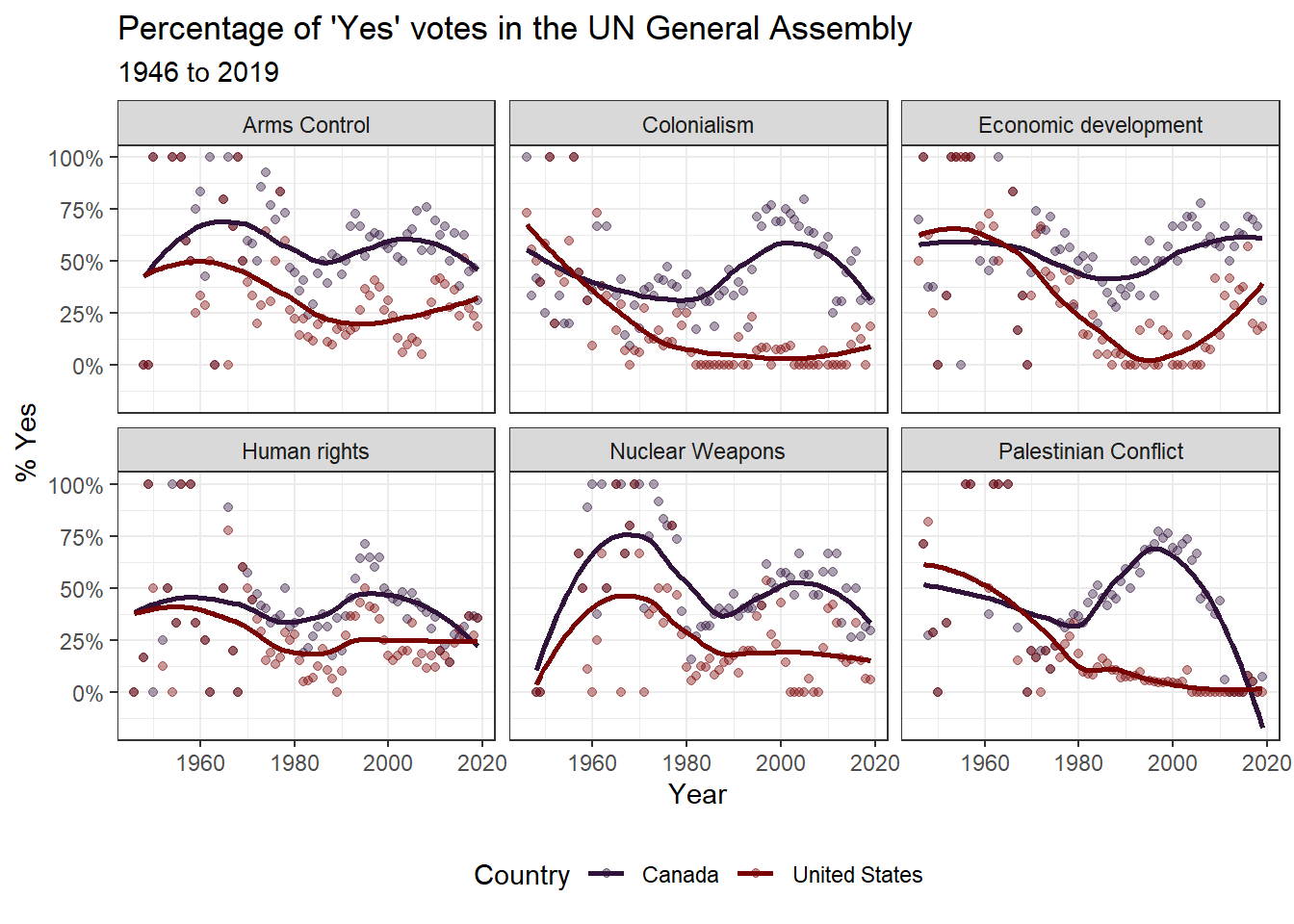
What do you notice about the voting records over time?
Demonstration: Adding more data
After your instructor created the above plot, she became curious about how politics might impact the UN Voting record for the United States since UN Ambassador is a presidential appointment. So your instructor started searching for a data set of US presidents, their years in office, and their political affiliation. She found a data set on Kaggle.com and removed the information prior to 1940 (because the dates were coded funny and it was causing problems). She saved the data as us_presidents.csv and imported it into the project.
president <- read_csv("data/us_presidents.csv", show_col_types = FALSE)
slice_sample(president, n = 10) |>
  gt() |>
tab_header(title = "president")| president | |||||||
|---|---|---|---|---|---|---|---|
| id | S.No. | start | end | president | prior | party | vice |
| 40 | 41 | 1/20/1989 | 20-Jan-93 | George H. W. Bush | 43rd Vice President of the United States | Republican | Dan Quayle |
| 25 | 26 | 9/14/1901 | 4-Mar-09 | Theodore Roosevelt | 25th Vice President of the United States | Republican | Office vacant |
| 33 | 34 | 1/20/1953 | 20-Jan-61 | Dwight D. Eisenhower | Supreme Allied Commander Europe ( 1949–1952 ) | Republican | Richard Nixon |
| 44 | 45 | 1/20/2017 | -- | Donald Trump | Chairman of The Trump Organization ( 1971–present ) | Republican | Mike Pence |
| 32 | 33 | 4/12/1945 | 20-Jan-53 | Harry S. Truman | 34th Vice President of the United States | Democratic | Office vacant |
| 26 | 27 | 3/4/1909 | 4-Mar-13 | William Howard Taft | 42nd United States Secretary of War (1904–1908) | Republican | James S. Sherman |
| 39 | 40 | 1/20/1981 | 20-Jan-89 | Ronald Reagan | 33rd Governor of California ( 1967–1975 ) | Republican | George H. W. Bush |
| 43 | 44 | 1/20/2009 | NA | Barack Obama | U.S. Senator ( Class 3 ) from Illinois ( 2005–2008 ) | Democratic | Joe Biden |
| 41 | 42 | 1/20/1993 | 20-Jan-01 | Bill Clinton | 40th & 42nd Governor of Arkansas (1979–1981 & 1983–1992) | Democratic | Al Gore |
| 27 | 28 | 3/4/1913 | 4-Mar-21 | Woodrow Wilson | 34th Governor of New Jersey (1911–1913) | Democratic | Thomas R. Marshall |
She realized that her data only had the start/end dates for each president and she wanted a data set that filled in the missing years and political party for the president in that time period. After much googling and reading Stack Overflow, found two functions she did not know about called complete() and fill() to fill in the missing years and party affiliations
politics_year <- president |>
    mutate(start = lubridate::mdy(start),  #formats date correctly
           start_year = lubridate::year(start)) |> #pulls out year
  filter(start_year > 1940) |>  #removes data before 1940 since there was no UN
  select(start_year, party) |>   #pulls out just the variables of interest
  complete(start_year = seq(min(start_year), 2020, by = 1)) |> #fill in missing years
  fill(party) #fill in missing party affiliations for years

slice_tail(politics_year, n = 10) |>
  gt() |>
tab_header(title = "Year by Presidential Party")| Year by Presidential Party | |
|---|---|
| start_year | party |
| 2011 | Democratic |
| 2012 | Democratic |
| 2013 | Democratic |
| 2014 | Democratic |
| 2015 | Democratic |
| 2016 | Democratic |
| 2017 | Republican |
| 2018 | Republican |
| 2019 | Republican |
| 2020 | Republican |
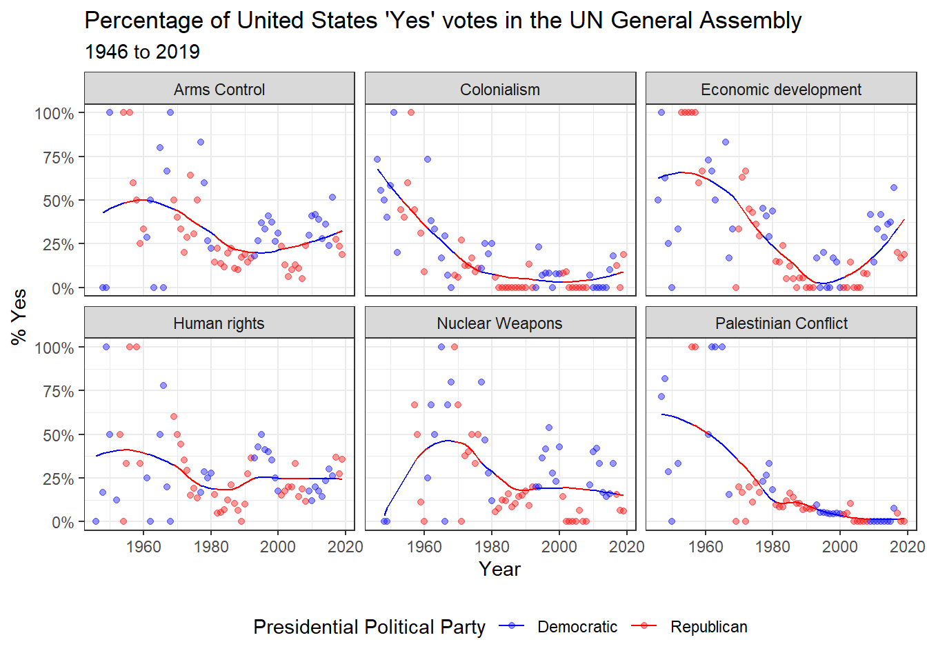
Next, your instructor took the yes_votes data and filtered out just the United States data and then joined by year to add the party affiliation of the president for each year of UN votes. To create the visualization with the smoothed model, but color by party affiliation, she had to add a new column called predict that fit the model first instead of using geom_smooth().
yes_votes |>
  filter(country == "United States") |>  #we want to focus on the US
  left_join(politics_year,
            by = c("year" = "start_year")) |> #adding in president political affiliation data
  group_by(issue) |>  #we want to calculate predicted yes by issue type
  mutate(predict = predict(loess(prop_yes ~ year))) |>  #creates predictions using a loess model for yes vs year
  ungroup() |> #ungroups the group_by line so it doesn't mess with other calculations
  ggplot(mapping = aes(x = year,
                       color = party,
                       group = 1)) + #sets universal aes to observe changes over time
  geom_point(aes(y = prop_yes),
             alpha = 0.4) + #plots points for proportion yes but transparent
  geom_line(aes(y = predict)) + #plots the predicted yeses for votes
  facet_wrap(~issue) + #creates a plot for each issue
  scale_y_continuous(labels = scales::percent) + #scales y-axis as percent values
  labs(
    title = "Percentage of United States 'Yes' votes in the UN General Assembly",
    subtitle = "1946 to 2019",
    y = "% Yes",
    x = "Year",
    color = "Presidential Political Party"
  ) + #adds labels
  theme_bw() + #changes appearance
  scale_color_manual(values = c("blue", "red"),
                     breaks = c("Democratic", "Republican")) + #sets specific colors for each party
  theme(legend.position = "bottom")  #moves legend to bottom to create space